Measuring Distance
Point to Point distance
In spatial analysis, we often want to know the shortest distance between two features. For example, we may want to know the distance from residence to pharmacy store to see if the distance affects people’s health. Or, we may be interested in whether the distance to airport or highway affects population growth. In this example, we will measure the nearest distance to airport in Pennsylvania, USA.
As usual, we need to import libraries we will be using.
[1]:
%matplotlib inline

import numpy as np
import pandas as pd
import geopandas as gpd
import matplotlib.pyplot as plt
Then, we load the example data and airport data and explore the data by plotting them together.
[2]:
df = pd.read_csv('../data/example.csv')
[3]:
from gps2space import geodf
gdf = geodf.df_to_gdf(df, x='longitude', y='latitude')
gdf.head()
[3]:
| pid | timestamp | latitude | longitude | geometry | |
|---|---|---|---|---|---|
| 0 | P2 | 2020-04-27 10:42:22.162176000 | 40.993799 | -76.669419 | POINT (-76.66942 40.99380) |
| 1 | P2 | 2020-06-02 01:12:45.308505600 | 39.946904 | -78.926234 | POINT (-78.92623 39.94690) |
| 2 | P2 | 2020-05-08 23:47:33.718185600 | 41.237403 | -79.252317 | POINT (-79.25232 41.23740) |
| 3 | P2 | 2020-04-26 14:31:12.100310400 | 41.991390 | -77.467769 | POINT (-77.46777 41.99139) |
| 4 | P2 | 2020-03-31 15:53:27.777897600 | 41.492674 | -76.542921 | POINT (-76.54292 41.49267) |
[4]:
airport = gpd.read_file('../data/paairport.shp')
airport.head()
[4]:
| STATE | NAME | geometry | |
|---|---|---|---|
| 0 | Pennsylvania | Erie International | POINT (-80.17600 42.08208) |
| 1 | Pennsylvania | Bradford Regional | POINT (-78.63987 41.80313) |
| 2 | Pennsylvania | Venango Regional | POINT (-79.86014 41.37793) |
| 3 | Pennsylvania | Wilkes-Barre/Scranton International | POINT (-75.72390 41.33823) |
| 4 | Pennsylvania | Williamsport Regional | POINT (-76.92144 41.24205) |
[5]:
pacounty = gpd.read_file('../data/pacounty.shp')
[6]:
ax = pacounty.boundary.plot(figsize=(12, 12), edgecolor='black', linewidth=0.6)
gdf.plot(ax=ax, color='r')
airport.plot(ax=ax, color='g', marker='*', markersize=60)

plt.show();
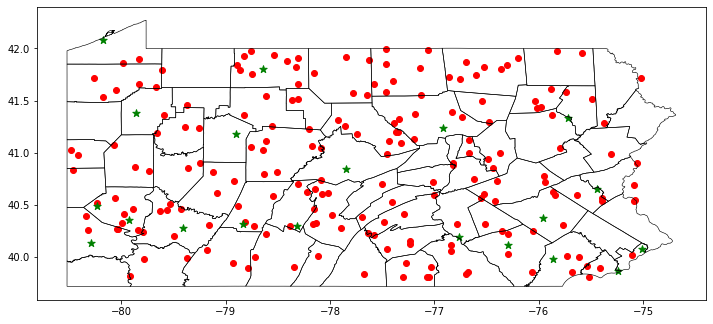
The red dots are the footprints of Person 1 (P1) and Person 2 (P2) while the green stars are the airports in Pennsylvania, USA.
We can calculate the distance from each point of P1 and P2 to the nearest airport using the dist_to_point function in the dist module. The dist_to_point function takes three parameters:
- gdf_a: This is the GeoDataFrame of P1 and P2’s footprints
- gdf_b: This is the landmark from where you want to measure the distance
- proj: This is the EPSG identifier you want to use to project your spatial data and will be applied to gdf_a and gdf_b
Because the airport data come from other source, we do not know if it has been projected or what is the projection system. So we want to check the projection system for airport data.
[7]:
airport.crs
It returns nothing, which means this data do not have projection. We will give it an initial projection of EPSG:4326.
[8]:
airport.crs = ("epsg:4326")
Now, we can import the dist function to calculate the distance from each point of P1 and P2 to the nearest airport.
[9]:
from gps2space import dist
[10]:
dist_to_airport = dist.dist_to_point(gdf, airport, proj=2163)
[11]:
dist_to_airport.head()
[11]:
| pid | timestamp | latitude | longitude | geometry | STATE | NAME | dist2point | |
|---|---|---|---|---|---|---|---|---|
| 0 | P2 | 2020-04-27 10:42:22.162176000 | 40.993799 | -76.669419 | POINT (1926745.083 -169042.499) | Pennsylvania | Williamsport Regional | 34579.711173 |
| 1 | P2 | 2020-06-02 01:12:45.308505600 | 39.946904 | -78.926234 | POINT (1774126.223 -333525.438) | Pennsylvania | Johnstown-Cambria County | 42187.331826 |
| 2 | P2 | 2020-05-08 23:47:33.718185600 | 41.237403 | -79.252317 | POINT (1712951.727 -200231.269) | Pennsylvania | Du Bois-Jefferson County | 30051.080354 |
| 3 | P2 | 2020-04-26 14:31:12.100310400 | 41.991390 | -77.467769 | POINT (1833671.313 -79623.054) | Pennsylvania | Williamsport Regional | 94804.346362 |
| 4 | P2 | 2020-03-31 15:53:27.777897600 | 41.492674 | -76.542921 | POINT (1921659.985 -112174.444) | Pennsylvania | Williamsport Regional | 42388.435141 |
The dist2point column represents the distance from each point to the nearest airport measured in meters. Likewise, you can then save the GeoDataFrame to a spatial dataset or non-spatial dataset as we did in the last section.
Point to Polygon distance
In this example, we want to calculate the nearest distance to parks represented in polygons using dist_to_poly function. The dist_to_poly function incorporates R-tree and spatial indexing technologies to boost the nearest neighbor query. The dist_to_poly function takes four parameters:
- gdf_source: This is the source GeoPandas dataframe
- gdf_target: This is the target GeoPandas dataframe
- proj: This is the EPSG identifier you want to use to project your spatial data and will be applied to gdf_source and gdf_target
- search_radius: This is the search radius in meters with a default value of None
Please note that:
- If
search_radiusis specified, points with no neighbors within the search radius, then thedist_to_polyfunction returns aNaNvalue - If
search_radiusis not specified, thedist_to_polyfunction employs brute-force search to find the nearest distance, and it may take longer time to calculate the nearest distance, especially for data in larger volumes
As usual, we read the park data as a GeoPandas dataframe. Then we illustrate how dist_to_poly works using two examples: an example specifying the search_radius and another example without specifying the search_radius
[12]:
park = gpd.read_file('../data/papark.shp')
park.head()
[12]:
| park_id | park_name | park_acres | geometry | |
|---|---|---|---|---|
| 0 | 1 | 11th Avenue Playground | 1.48 | POLYGON ((-79.89948 40.40552, -79.89946 40.406... |
| 1 | 22 | Alpine Parklet | 0.12 | POLYGON ((-80.01282 40.45765, -80.01303 40.457... |
| 2 | 6117 | Negley Park | 18.46 | POLYGON ((-76.89575 40.25092, -76.89178 40.249... |
| 3 | 8202 | Deer Lake Community Park | 32.76 | MULTIPOLYGON (((-76.05700 40.62615, -76.05696 ... |
| 4 | 8215 | Delano Playground | 1.37 | POLYGON ((-75.97098 40.80281, -75.97062 40.801... |
Specifying search_radius
[13]:
%%time
dist_with_search_radius = dist.dist_to_poly(gdf, park, proj=2163, search_radius=10000)
A search_radius of 10000 meters is specified. Points with no neighbors intersected with thte search radius will return NaN.
Wall time: 4.57 s
[14]:
dist_with_search_radius
[14]:
| pid | timestamp | latitude | longitude | geometry | dist2poly | |
|---|---|---|---|---|---|---|
| 0 | P2 | 2020-04-27 10:42:22.162176000 | 40.993799 | -76.669419 | POINT (1926745.083 -169042.499) | 3143.431951 |
| 1 | P2 | 2020-06-02 01:12:45.308505600 | 39.946904 | -78.926234 | POINT (1774126.223 -333525.438) | 4007.426442 |
| 2 | P2 | 2020-05-08 23:47:33.718185600 | 41.237403 | -79.252317 | POINT (1712951.727 -200231.269) | 7198.553223 |
| 3 | P2 | 2020-04-26 14:31:12.100310400 | 41.991390 | -77.467769 | POINT (1833671.313 -79623.054) | 4418.972172 |
| 4 | P2 | 2020-03-31 15:53:27.777897600 | 41.492674 | -76.542921 | POINT (1921659.985 -112174.444) | 4997.223163 |
| ... | ... | ... | ... | ... | ... | ... |
| 195 | P1 | 2020-04-14 22:59:47.187801600 | 40.592932 | -77.002548 | POINT (1912029.573 -220204.526) | 2789.935358 |
| 196 | P1 | 2020-02-18 16:00:05.505350400 | 40.263436 | -80.322911 | POINT (1651469.678 -328218.968) | 3433.440261 |
| 197 | P1 | 2020-02-24 10:22:29.605353600 | 40.726640 | -76.403706 | POINT (1956064.504 -191577.975) | 6104.559787 |
| 198 | P1 | 2020-01-13 10:02:15.962697600 | 40.279678 | -77.898978 | POINT (1848682.909 -274721.379) | 2696.384797 |
| 199 | P1 | 2020-04-02 23:09:49.639881600 | 41.660656 | -79.830351 | POINT (1655332.627 -166134.557) | 5926.050348 |
200 rows × 6 columns
Without specifying search_radius
[15]:
%%time
dist_no_search_radius = dist.dist_to_poly(gdf, park, proj=2163)
No search_radius is specified, the calculation may take longer time for datasets in large volumes.
Wall time: 17.3 s
[16]:
dist_no_search_radius
[16]:
| pid | timestamp | latitude | longitude | geometry | dist2poly | |
|---|---|---|---|---|---|---|
| 0 | P2 | 2020-04-27 10:42:22.162176000 | 40.993799 | -76.669419 | POINT (1926745.083 -169042.499) | 3143.431951 |
| 1 | P2 | 2020-06-02 01:12:45.308505600 | 39.946904 | -78.926234 | POINT (1774126.223 -333525.438) | 4007.426442 |
| 2 | P2 | 2020-05-08 23:47:33.718185600 | 41.237403 | -79.252317 | POINT (1712951.727 -200231.269) | 7198.553223 |
| 3 | P2 | 2020-04-26 14:31:12.100310400 | 41.991390 | -77.467769 | POINT (1833671.313 -79623.054) | 4418.972172 |
| 4 | P2 | 2020-03-31 15:53:27.777897600 | 41.492674 | -76.542921 | POINT (1921659.985 -112174.444) | 4997.223163 |
| ... | ... | ... | ... | ... | ... | ... |
| 195 | P1 | 2020-04-14 22:59:47.187801600 | 40.592932 | -77.002548 | POINT (1912029.573 -220204.526) | 2789.935358 |
| 196 | P1 | 2020-02-18 16:00:05.505350400 | 40.263436 | -80.322911 | POINT (1651469.678 -328218.968) | 3433.440261 |
| 197 | P1 | 2020-02-24 10:22:29.605353600 | 40.726640 | -76.403706 | POINT (1956064.504 -191577.975) | 6104.559787 |
| 198 | P1 | 2020-01-13 10:02:15.962697600 | 40.279678 | -77.898978 | POINT (1848682.909 -274721.379) | 2696.384797 |
| 199 | P1 | 2020-04-02 23:09:49.639881600 | 41.660656 | -79.830351 | POINT (1655332.627 -166134.557) | 5926.050348 |
200 rows × 6 columns
[18]:
dist_no_search_radius[dist_no_search_radius['dist2poly'] == 'NaN']
[18]:
| pid | timestamp | latitude | longitude | geometry | dist2poly |
|---|
[23]:
dist_with_search_radius.describe().T
[23]:
| count | mean | std | min | 25% | 50% | 75% | max | |
|---|---|---|---|---|---|---|---|---|
| latitude | 200.0 | 40.878765 | 0.649778 | 39.807771 | 40.321969 | 40.821446 | 41.468584 | 41.991390 |
| longitude | 200.0 | -77.732011 | 1.465171 | -80.485216 | -78.824666 | -77.635756 | -76.549980 | -75.025528 |
| dist2poly | 185.0 | 3919.033243 | 2802.089284 | 0.000000 | 1550.077077 | 3623.525457 | 5316.719387 | 13855.516463 |
[20]:
dist_no_search_radius.describe().T
[20]:
| count | mean | std | min | 25% | 50% | 75% | max | |
|---|---|---|---|---|---|---|---|---|
| latitude | 200.0 | 40.878765 | 0.649778 | 39.807771 | 40.321969 | 40.821446 | 41.468584 | 41.991390 |
| longitude | 200.0 | -77.732011 | 1.465171 | -80.485216 | -78.824666 | -77.635756 | -76.549980 | -75.025528 |
| dist2poly | 200.0 | 4726.981887 | 4027.497246 | 0.000000 | 1849.390860 | 3877.189734 | 5970.677707 | 21244.390382 |
The above results show that specifying a search radius decreases the time needed for the nearest distance calculation, and most of the points have neighbors within the search radius, the final results are similar.